前言
本文的主体是Ian Goodfellow 「Deep Learning」第五章「MACHINE LEARNING BASICS」,未经动手实做,故称纸上谈兵。目前奉行Lazy evaluation,对相关知识的补充会在实践后进行。
what is machine learning
A computer program is said to learn from experience E with respect to some class of tasks T and performance measure P, if its performance at tasks in T, as measured by P, improves with experience E
The Task T
- Classification
- Regression
- Structured output
The performance measure P
Usually we are interested in how well the machine learning algorithm performs on data that it has not seen before, since this determines how well it will work when deployed in the real world. We therefore evaluate these performance measures using a test set of data that is separate from the data used for training the machine learning system.
It’s often difficult to choose a performance measure that corresponds well to the desired behavior of the system for two reasons
- The performance measure can be difficult to decide. When performing a regression task, should we penalize the system more if it frequently makes medium-sized mistakes or if it rarely makes very large mistakes? These kinds of design choices depend on the application
- we know what quantity we would ideally like to measure, but measuring it is impractical. Computing the actual probability value assigned to a specific point in space in many density estimation models is intractable
The Experience E
Machine learning algorithms can be broadly categorized as unsupervised or supervised by what kind of experience they are allowed to have during the learning process.
- Unsupervised learning algorithms experience a dataset containing many features, then learn useful properties of the structure of this dataset. In the context of deep learning, we usually want to learn the entire probability distribution that generated a dataset, whether explicitly as in density estimation or implicitly for tasks like synthesis or denoising. Some other unsupervised learning algorithms perform other roles, like clustering, which consists of dividing the dataset into clusters of similar examples.
- Supervised learning algorithms experience a dataset containing features,but each example is also associated with a label or target.
Roughly speaking, unsupervised learning involves observing several examples
of a random vector x, and attempting to implicitly or explicitly learn the probability distribution p(x), or some interesting properties of that distribution, while supervised learning involves observing several examples of a random vector x and an associated value or vector y, and learning to predict y from x, usually by estimating p(y|x) The term supervised learning originates from the view of the target y being provided by an instructor or teacher who shows the machine learning system what to do. In unsupervised learning, there is no instructor or teacher, and the algorithm must learn to make sense of the data without this guide
Some machine learning algorithms do not just experience a fixed dataset. For example, reinforcement learning algorithms interact with an environment, so there is a feedback loop between the learning system and its experiences
Example: Linear regression
- The task T: linear regression solves a regression problem. The goal is to build a system that can take a vector x ∈ R^n as input and predict the value of a scalar y ∈ R as its output.
w is a vector of the weights over different features.
b is the bias(not the bias in statistic)
Together ,w and b are called the parameters
y is the label of the data.
y-hat is the prediction value
- The performance measurement P:
mean squared error(MSE)
$$\mathrm{MSE_{test}}=\frac{1}{m}\sum_i(\hat{y}^{(test)}-y^{(test)})$$Capacity, Overfitting and Underfitting
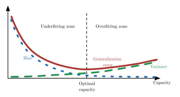
The central challenge in machine learning is that we must perform well on new, previously unseen inputs—not just those on which our model was trained. The ability to perform well on previously unobserved inputs is called generalization.
The factors determining how well a machine learning algorithm will perform are its ability to:
- Make the training error small.
- Make the gap between training and test error small.
These two factors are underfitting and overfitting. Underfitting occurs when the model is not able to obtain a sufficiently low error value on the training set. Overfitting occurs when the gap between the training error and test error is too large.
Informally, a model’s capacity is its ability to fit a wide variety of functions. Models with low capacity may struggle to fit the training set. Models with high capacity can overfit by memorizing properties of the training set that do not serve them well on the test set. Usually,the error mainly comes from bias in the case of underfitting and variance in the case of overfitting.
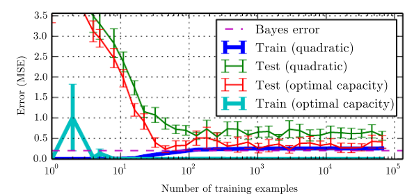
Bayes error
The error incurred by an oracle making predictions from the true distribution
p(x,y) is called the Bayes error.
Why are there errors if we know the true probability distribution ?
because there may still be some noise in the distribution
How about training size
Training and generalization error vary as the size of the training set varies.
Expected generalization error can never increase as the number of training examples increases. For non-parametric models, more data yields better generalization until the best possible error is achieved. Any fixed parametric model with less than optimal capacity will asymptote to an error value that exceeds the Bayes error. See figure
5.4 for an illustration. Note that it is possible for the model to have optimal
capacity and yet still have a large gap between training and generalization error. In this situation, we may be able to reduce this gap by gathering more training examples.
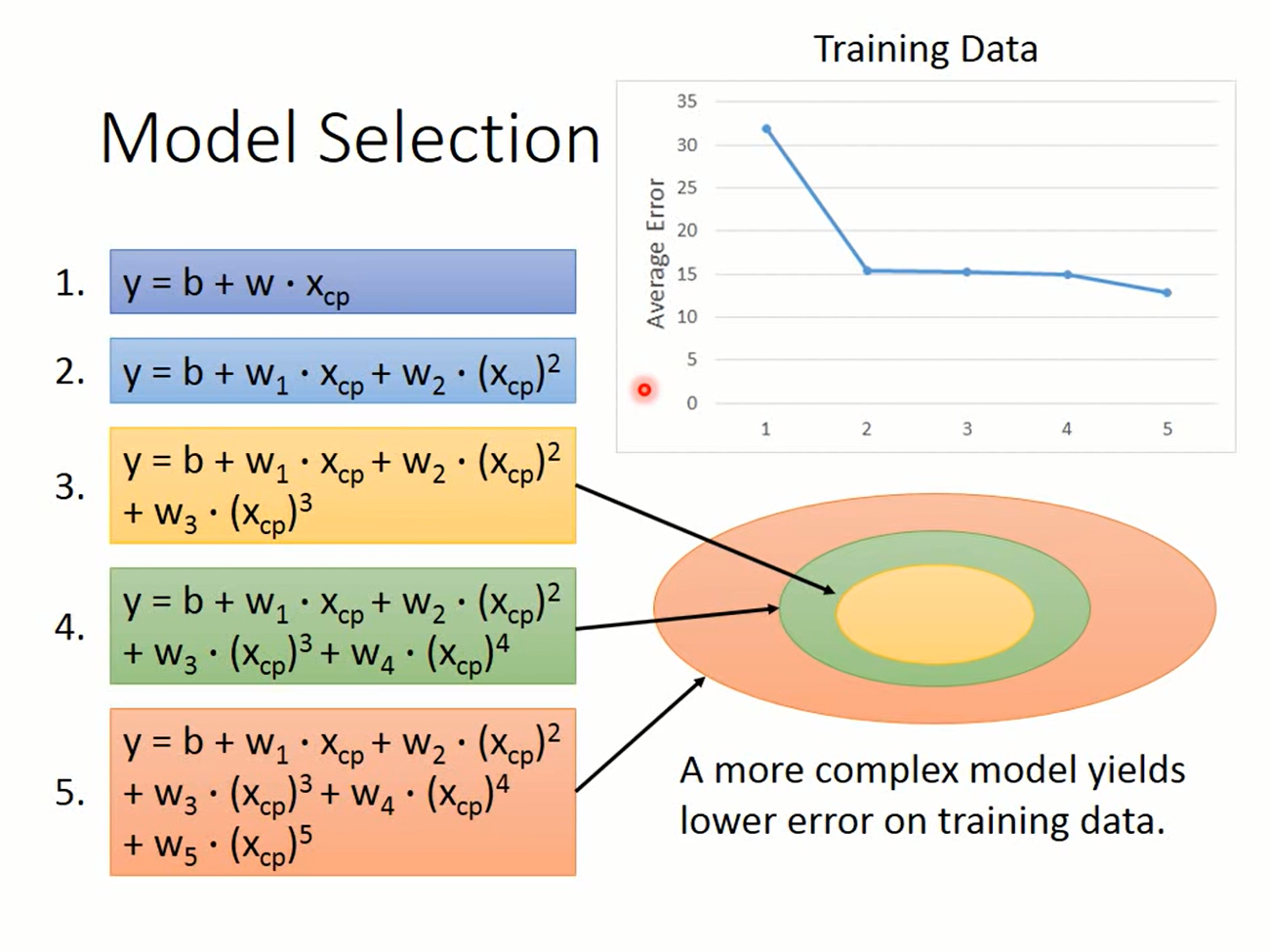
Hyperparameters
hyperparameters are use to control the behavior of the learning algorithm.
Eg. In linear regression, we could use a model
$$\hat{y}=b+\sum_i^kw_ix^i$$k controls degree of the polynomial,which acts as a capacity hyperparameter
Why hyperparameters?
Sometimes a setting is chosen to be a hyperparameter that the learning algorithm does not learn because it is difficult to optimize. The setting must be a hyperparameter because it is not appropriate to learn that hyperparameter on the training set. This applies to all hyperparameters that control model capacity(e.g:k). If learned on the training set, such hyperparameters would always choose the maximum possible model capacity, resulting in overfitting
How to adjust hyperparameters?
Validation set!
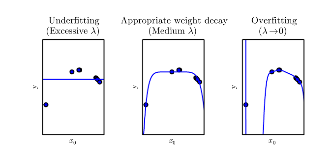
Regularization
We can give a learning algorithm a preference for one solution in its hypothesis space to another. This means that both functions are eligible, but one is preferred.(即西瓜书提到的归纳假设)
For example, we can modify the training criterion for linear regression to include weight decay
$$J(w)=\mathrm{MSE_{train}}+\lambda w^\top w$$where λ is a value chosen ahead of time that controls the strength of our preference for smaller weights. in this sense, λ is also a hyperparameter
Frequentist vs baysian
- Frequentist statistics: we assume that the true parameter value θ is fixed but unknown, while the point estimate θ_hat is a function of the data. Since the data is drawn from a random process, any function of the data is random. Therefore θ_hat is a random variable
- Bayesian Statistics: the dataset is directly observed and so is not random. On the other hand, the true parameter θ is unknown or uncertain and thus is represented as a random variable. Before observing the data, we represent our knowledge of θ using the prior probability distribution, p(θ). Generally, the machine learning practitioner selects a prior distribution that is quite broad (i.e. with high entropy) to reflect a high degree of uncertainty in the value of θ before observing any data
Maximum likelihood
|
|
The maximum likelihood estimator for is defined as
$$\theta_{ML}=\argmax _\theta\prod_{i=1}^mp_{model}(x^i;\theta)$$log-likelihood estimator
$$\theta_{ML}=\argmax _\theta\sum_{i=1}^m\log p_{model}(x^i;\theta)$$观察KL-Divergence:
$$D_{KL}(\hat{p}_{data}\|p_{model})=\mathbb{E}_{x\sim \hat{p}_{data}}[\log \hat{p}_{data}(x) - \log \hat{p}_{model}(x)]$$为了最小化KL-Divergence,只需最小化
$$- \mathbb{E}_{x\sim \hat{p}_{data}} \log \hat{p}_{model}(x)]$$这与最大化log-likelihood是等价的
Simple machine learning algorithm
SVM
One of the most influential approaches to supervised learning is the support vector machine This model is similar to logistic regression in that it is driven by a linear function
$$y=w^\top x+b$$. The SVM predicts that the positive class is present when y is positive. Likewise, it predicts that the negative class is present when y is negative.
One key innovation associated with support vector machines is the kernel trick. The kernel trick consists of observing that many machine learning algorithms can be written exclusively in terms of dot products between examples. For example, it can be shown that the linear function used by the support vector machine can be re-written as
$$w^\top x+b=b+\sum_i^m \alpha_i x^\top x^{(i)}$$where x^i is a training example and α is a vector of coefficients.Rewriting the learning algorithm this way allows us to replace x by the output of a given feature function φ(x) and the dot product with a function k(x,x^i) = φ(x)· φ(x^i) called a kernel.
The most commonly used kernel is the Gaussian kernel
$$k(u,v)=\mathbin{N}(u-v;0;\sigma^2I)$$this kernel is also known as the radial basis function (RBF) kernel. The Gaussian kernel is performing a kind of template matching. A training example x associated with training label y becomes a template for class y. When a test point x’ is near x according to Euclidean distance, the Gaussian kernel has a large response, indicating that x’ is very similar to the x template. The model then puts a large weight on the associated training label y. Overall, the prediction will combine many such training labels weighted by the similarity of the corresponding training examples
Gradient descent improved: stochastic gradient descent
Idea:
- take a step over a ‘minibatch’ instead of observing the whole training-set
- step cost does not depend on size of training set, thus achieving convergence much faster.
A recurring problem in machine learning is that large training sets are necessary for good generalization, but large training sets are also more computationally expensive.
the insight of stochastic gradient descent is that the gradient is an expectation. The expectation may be approximately estimated using a small set of samples. Specifically, on each step of the algorithm, we can sample a minibatch of examples
For a fixed model size, the cost per SGD update does not depend on the training set size m. In practice, we often use a larger model as the training set size increases, but we are not forced to do so. The number of updates required to reach convergence usually increases with training set size. However, as m approaches infinity, the model will eventually converge to its best possible test error before SGD has sampled every example in the training set. Increasing m further will not extend the amount of training time needed to reach the model’s best possible test error. From this point of view, one can argue that the asymptotic cost of training a model with SGD is O(1) as a function of m
Why deep learning?
curse of dimensionality
Many machine learning problems become exceedingly difficult when the number of dimensions in the data is high.
| dimension | number of states |
|---|---|
| 1 | n |
| 2 | n^2 |
| 3 | n^3 |
Traditional machine learning algorithm can’t distinguish a state that’s not seen in the training set.
Local Constancy and Smoothness Regularization
In order to generalize well, machine learning algorithms need to be guided by prior beliefs about what kind of function they should learn.
Among the most widely used of these implicit “priors” is the smoothness prior or local constancy prior. This prior states that the function we learn should not change very much within a small region. Many simpler algorithms rely exclusively on this prior to generalize well, and as a result they fail to scale to the statistical challenges involved in solving AIlevel tasks.
How do we deal with curse of dimensionality?
The key insight is that a very large number of regions, e.g., O(2^k), can be defined with O(k) examples, so long as we introduce some dependencies between the regions via additional assumptions about the underlying data generating distribution
The core idea in deep learning is that we assume that the data was generated by the composition of factors or features, potentially at multiple levels in a hierarchy.
Manifold Learning & manifold hypothesis
Manifold learning algorithms assuming that most of R^n consists of invalid inputs, and that interesting inputs occur only along a collection of manifolds containing a small subset of points.
manifold hypothesis:
-
probability distribution over images, text strings, and sounds that occur in real life is highly concentrated.
-
we can also imagine such neighborhoods and transformations, at least informally. In the case of images, we can certainly think of many possible transformations that allow us to trace out a manifold in image space: we can gradually dim or brighten the lights, gradually move or rotate objects in the image, gradually alter the colors on the surfaces of objects
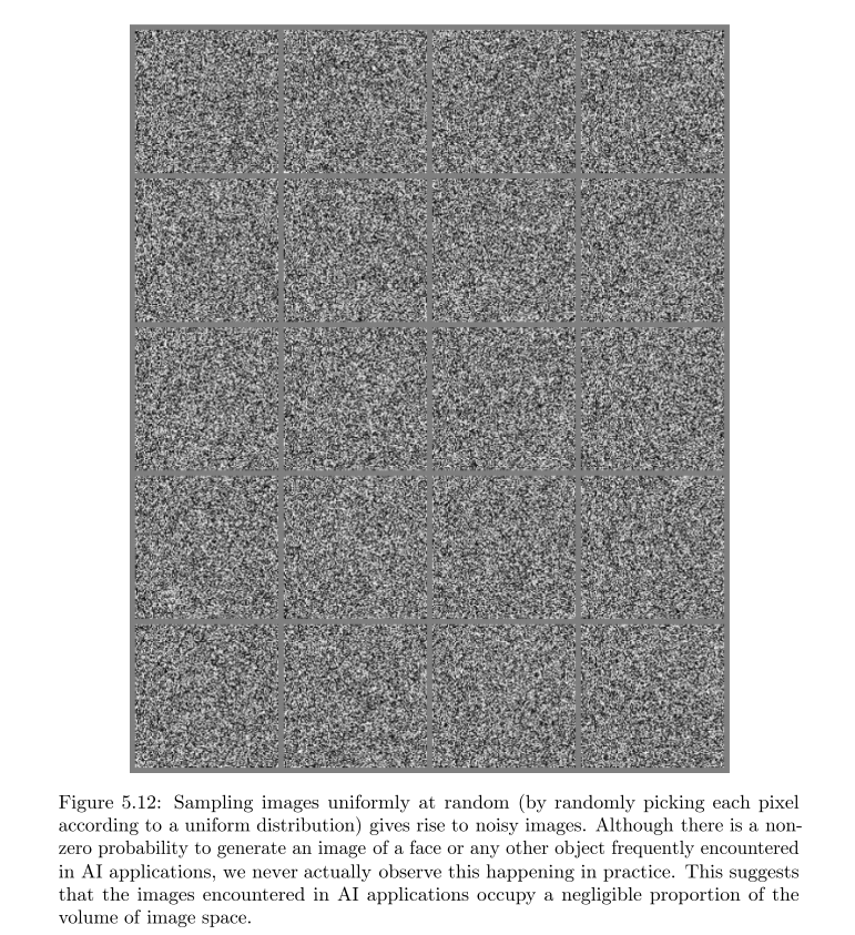
流形假说:
- 大部分有结构的数据的分布函数并不是分散的,而是集中聚集在某些范围。
支持证据:随机取像素试图产生而期待其产生日常生活中的照片的概率是微乎其微的。随机取字母指望它生成一篇文章的概率也是微乎其微的。所以有结构的数据的分布函数必然是在某个范围内聚集,而在大部分区域分散
- 在流形的表面移动,将可以得到流形所代表的全部数据。如在代表人脸的流形上移动,A点代表微笑的人,B点代表流泪的人。若从直线直接过去,则在A,B中间点所对应的数据可能不是人脸;若从流形的表面移动到B,则数据一直都是人脸。(微笑->皱眉->哭泣)
请参考Youtube视频:My understanding of the Manifold Hypothesis | Machine learning