Deep learning algorithms are typically applied to extremely complicated domains where the true generation process essentially involves simulating the entire universe… Controlling the complexity of the model is not a simple matter of finding the model of the right size, with the right number of parameters. Instead, we might find—and indeed in practical deep learning scenarios, we almost always do find—that the best fitting model (in the sense of minimizing generalization error) is a large model that has been regularized appropriately
regularization是我们应对overfitting的常用手段。在比较简单的模型,例如linear-regresseion中,人对的capacity的估计通常比较准确,一般不需要做regularization。而在神经网络动辄成千上万个节点,数以百万的参数让估测capacity变得极为困难。正如花书所说,泛化性能最好的往往是复杂的模型加上合理的regularization而得到的
Parameter Penalities
正如三次式最高次的系数为零时退化为二次式,有越多的参数接近0,模型的capacity就越低,即「绑住手脚」。一般来说regularization不会考虑bias,因为bias对capacity的影响并不如weight那么大,但有需要仍可以给bias加上惩罚。
参数惩罚的思路是,给Loss加上所有参数θ的函数Ω(θ)这一项,让模型更偏好于θ接近0的归纳假设。
L2 norm
L2 norm中所选的函数Ω是
$$\Omega(\theta)=\frac{1}{2}\theta^{\top}\theta$$Loss的梯度变为
带入梯度下降公式
$$ \theta^{N+1} \leftarrow\theta^N-\epsilon\nabla_\theta \hat{L} =\theta^N-\epsilon\nabla_\theta L - \alpha\epsilon \theta^N = (1-\alpha \epsilon)\theta ^N-\epsilon\nabla_\theta L $$每次梯度下降更新参数时会把原来的参数乘上一个固定的值1-αε,使得θ接近于0
L1 norm
L1 norm中的函数Ω是
$$ \Omega(\theta)=\sum_{i=1}^N|\theta_i| $$
Loss的梯度变为
带入梯度下降公式
$$ \theta^{N+1} \leftarrow\theta^N-\epsilon\nabla_\theta \hat{L} =\theta^N-\epsilon\nabla_{\theta}L-\alpha\epsilon \mathrm{sgn}(\theta^N) = \theta ^N-\epsilon\nabla_\theta L -\alpha\epsilon \mathrm{sgn}(\theta^N) $$发现参数更新时会在每一个分量i中减掉一个固定值αε*sgn(i)
L2 norm中,每次都乘上一个小于1的数,当参数大于1时,减小的速度就非常快;当参数小于1时,减小的速度就比较慢。因此L2中最终各个参数比较接近,但不会出现很多0。
而L1 norm中,每次减小一个固定值。对很大的参数,减法的步长很小,减小的效果就不是很明显。而参数很小时,减法的步长相对很大,就很容易出现0。因此L1中很容易出现很大的参数和较多的0。
含较多0的矩阵叫做稀疏矩阵(Sparse matrix),因此用L1能够得到比较稀疏的参数。
Early stopping
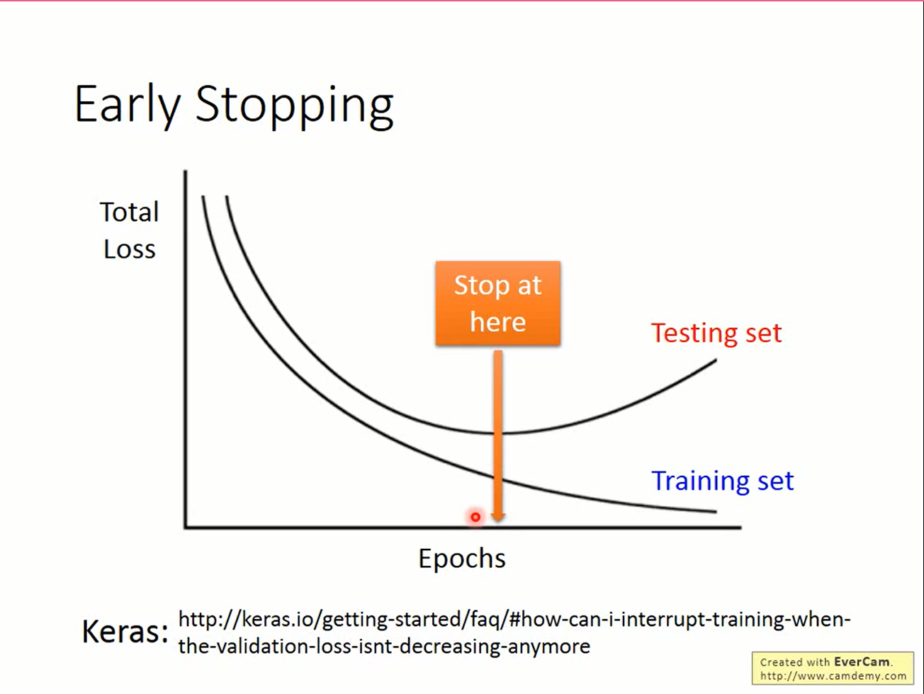
early stopping的思路就更简单了。既然复杂的模型训练时会关注一些无关的特征,那干脆不要跑那么多次训练就好了。
early stopping的形式化描述:
|
|
|
|
Ensemble
Ensemble认为,模型中出现的错误是随机的,那么使用同样的数据训练出k个不同的模型,将它们的结果取平均就可以得到比较好的结果。
复杂模型error主要来自variance。从直觉上说,对多个模型取平均就能很好的抵消一部分variance。 ensemble的坏处在于,它需要训练k个不同的模型,导致计算量大增。有时这样的计算量是无法承受的,因此希望有一个代价不那么大的ensemble方法,这就是dropout
dropout
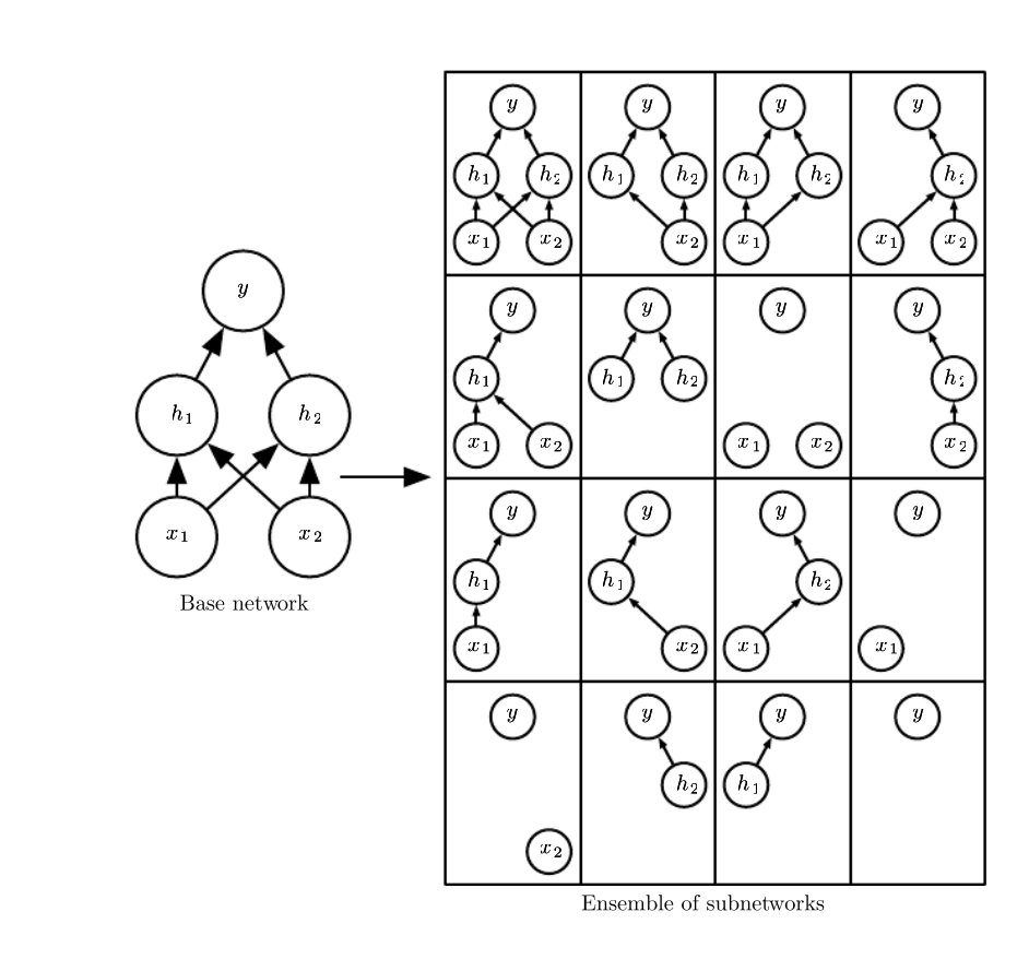
dropout和以往的方法不同,它把当前训练的模型当作是很多模型的叠加:每次训练时,每个单元都有p的概率从网络中被移除,每次只针对这些被留下来的单元做参数的更新。有n个单元时,因为每一个单元都可以被留下/丢掉,这就可能产生2^N个不同的网络结构。dropout就认为当前的模型是这2^N个网络的ensemble。
下面是一个2层的神经网络。它有2个隐藏单元。dropout可以产生的网络由16个。使用dropout的网络经过一次训练后相当于训练了2^N个子网络,计算量的问题就这样解决了。
使用dropout的网络训练完成后,在测试时不再移除神经元,而是给网络整体的参数乘上1-p。 一个直觉的解释:
|
|
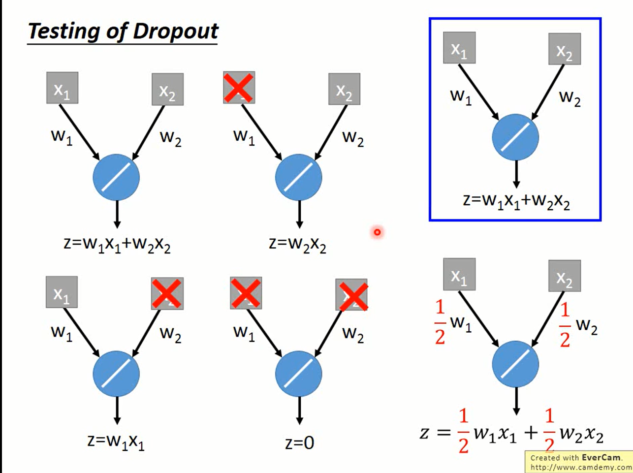
实际的分析发现,在整个网络是线性时,上面的论述是精确成立的,而加上激活函数的网络往往不是线性的。但实际使用上dropout的性能也确实比较接近ensemble的结果。为什么会这样我们不清楚,总之拿来主义了。世界各地有很多科学家也在探究背后的奥秘,希望有一天能找出一个精确的解释吧。